Hey everyone,

in the easter holidays I have challenged myself with a little numerical analysis problem. So I tried to write a program that interpolates points in a two dimensional plane.

What it is used for

Before we can figure out what interpolation can be used for, we first have to clear out, what interpolation is.

In the world of computers almost everything is discrete. For example, if we have a path a robot should take, such a path will probably be described by a set of waypoints. If the path should be 100% defined, we would need an infinite amount of waypoints. That would be impracticable.

A better way is to search for a function, that takes a finite set of waypoints and returns waypoints that could be in between the original set.

Polynomial Interpolation

A cubic function can do the trick. Such a function $f$ can be described by $ax^3+bx^2+cx+d$, where $a, b, c, d$ are parameters that have to be found by an algorithm. New datapoints (or waypoints) can be interpolated by $y = f(x)$. Like I said before, there are four parameters that have to be found, therefore we need at least four linear equations to find these parameters.

To get these linear equations we have to look at the way the given datapoints interact with the cubic function. The set of datapoints $x_i, y_i$ can be described with the function f so that $x_i = f(y_i),\;i \in{1, 2, …, n}$. So to get four of these equations we need at least four datapoints.

We can write that in an matrix equation.

\[\begin{bmatrix} x_1^3 &x_1^2 &x_1 &1 \\ x_2^3 &x_2^2 &x_2 &1 \\ \vdots &\vdots &\vdots &\vdots \\ x_n^3 &x_n^2 &x_n &1 \end{bmatrix} \begin{bmatrix} a\\ b\\ c\\ d \end{bmatrix} = \begin{bmatrix} y_1\\ y_2\\ \vdots\\ y_n \end{bmatrix}\]

There are a lot of ways and programs that can solve a linear equations like that. The left matrix is called a Vandermonde matrix. There are way better ways for generating a polynomial function but this is the most understandable way in my opinion. And just like that we can get the four parameter for the cubic function.

Now we can get a bunch of waypoints/datapoints by generating x coordinates and pass them in the function f.

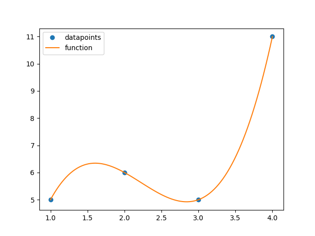
However there are some major problems with this method. The function starts to oscillate when more than four datapoints are provided.

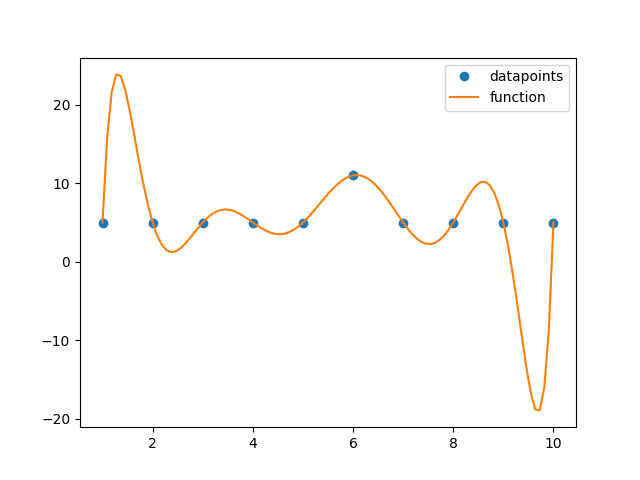
Take a look at how the function oscillates at the end of each side.
Imagine a robot tries to follow a path represented by these datapoints. You would expect the robot to move in a almost straight line (except a little curve in the middle). The problem is that the robot would destroy almost everything in its environment, especially in the beginning and in the end of its mission.

This problem can be solved by using a cubic spline.

Spline interpolation

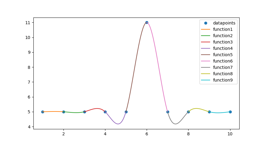
A spline is a piecewise polynomial function. So for each datapoint pair (e.g. $\{(x_0, y_0), (x_1, y_1)\},\{(x_1, y_1), (x_2, y_2)\},\dots,\{(x_{n-1}, y_{n-1}), (x_n, y_n)\}$) there is a function which connects these pairs. So for $n$ datapoints we need $n-1$ functions, like you can see in the graph below. Note that the datapoints in the graph are the same as the datapoints in the problematic graph above. You can already see, that the spline interpolation gets rid of the oscillation problem.

But if we just use the methods from the previous chapter we would end with two equations for each function. That is not enough to get our four coefficients. So we need two more equations for that.

To make sure that the transition between two functions is smooth, the fist and the second derivative on each function pair should be equal.

\[f'_i(x_{i+1}) = f'_{i+1}(x_{i+1})\] \[f''_i(x_{i+1}) = f''_{i+1}(x_{i+1})\]

Note that the equations above can be written as:

\[f'_i(x_{i+1}) - f'_{i+1}(x_{i+1}) = 0\] \[f''_i(x_{i+1}) - f''_{i+1}(x_{i+1}) = 0\]

So besides of the first and the last, every function has four equations.

We also want to make sure that our spline begins and fades out smoothly. For that, we have to ensure that the second derivative in the first and last datapoint is zero.

\[f''_1(x_1) = 0\] \[f''_{n-1}(x_n) = 0\]

As we see, we now have four equations for every function in the spline. So we can now determine our four coefficients for each function with the help of the linear equation system.

I tried my best to write that down in a matrix equation.

\[\begin{bmatrix} &x_1^3 &x_1^2 &x_1 &1 &0 &0 &0 &0 &0 &0 &0 &0 &\cdots &0 &0 &0 &0 &0 &0 &0 &0\\ &x_2^3 &x_2^2 &x_2 &1 &0 &0 &0 &0 &0 &0 &0 &0 &\cdots &0 &0 &0 &0 &0 &0 &0 &0\\ &0 &0 &0 &0 &x_2^3 &x_2^2 &x_2 &1 &0 &0 &0 &0 &\cdots &0 &0 &0 &0 &0 &0 &0 &0\\ &0 &0 &0 &0 &x_3^3 &x_3^2 &x_3 &1 &0 &0 &0 &0 &\cdots &0 &0 &0 &0 &0 &0 &0 &0\\ &0 &0 &0 &0 &0 &0 &0 &0 &x_3^3 &x_3^2 &x_3 &1 &\cdots &0 &0 &0 &0 &0 &0 &0 &0\\ &0 &0 &0 &0 &0 &0 &0 &0 &x_4^3 &x_4^2 &x_4 &1 &\cdots &0 &0 &0 &0 &0 &0 &0 &0\\ & & & & & & & & & & &\vdots & & & & & & & & & &\\ &0 &0 &0 &0 &0 &0 &0 &0 &0 &0 &0 &0 &\cdots &x_{n-2}^3 &x_{n-2}^2 &x_{n-2} &1 &0 &0 &0 &0\\ &0 &0 &0 &0 &0 &0 &0 &0 &0 &0 &0 &0 &\cdots &x_{n-1}^3 &x_{n-1}^2 &x_{n-1} &1 &0 &0 &0 &0\\ &0 &0 &0 &0 &0 &0 &0 &0 &0 &0 &0 &0 &\cdots &0 &0 &0 &0 &x_{n-1}^3 &x_{n-1}^2 &x_{n-1 } &1\\ &0 &0 &0 &0 &0 &0 &0 &0 &0 &0 &0 &0 &\cdots &0 &0 &0 &0 &x_{n}^3 &x_{n}^2 &x_{n} &1\\ &3x_2^2 &2x_2 &1 &0 &-3x_2^2 &-2x_2 &-1 &0 &0 &0 &0 &0 &\cdots &0 &0 &0 &0 &0 &0 &0 &0\\ &6x_2 &2 &0 &0 &-6x_2 &-2 &0 &0 &0 &0 &0 &0 &\cdots &0 &0 &0 &0 &0 &0 &0 &0\\ &0 &0 &0 &0 &3x_3^2 &2x_3 &1 &0 &-3x_3^2 &-2x_3 &-1 &0 &\cdots &0 &0 &0 &0 &0 &0 &0 &0\\ &0 &0 &0 &0 &6x_3 &2 &0 &0 &-6x_3 &-2 &0 &0 &\cdots &0 &0 &0 &0 &0 &0 &0 &0\\ &0 &0 &0 &0 &0 &0 &0 &0 &3x_4^2 &2x_4 &1 &0 &\cdots &0 &0 &0 &0 &0 &0 &0 &0\\ &0 &0 &0 &0 &0 &0 &0 &0 &6x_4 &2 &0 &0 &\cdots &0 &0 &0 &0 &0 &0 &0 &0\\ & & & & & & & & & & &\vdots & & & & & & & & & &\\ &0 &0 &0 &0 &0 &0 &0 &0 &0 &0 &0 &0 &\cdots &-3x_{n-2}^2 &-2x_{n-2} &-1 &0 &0 &0 &0 &0\\ &0 &0 &0 &0 &0 &0 &0 &0 &0 &0 &0 &0 &\cdots &-6x_{n-2} &-2 &0 &0 &0 &0 &0 &0\\ &0 &0 &0 &0 &0 &0 &0 &0 &0 &0 &0 &0 &\cdots &3x_{n-1}^2 &2x_{n-1} &1 &0 &-3x_{n-1}^2 &-2x_{n-1} &-1 &0\\ &0 &0 &0 &0 &0 &0 &0 &0 &0 &0 &0 &0 &\cdots &6x_{n-1} &2 &0 &0 &-6x_{n-1} &-2 &0 &0\\ &6x_1 &2 &0 &0 &0 &0 &0 &0 &0 &0 &0 &0 &\cdots &0 &0 &0 &0 &0 &0 &0 &0\\ &0 &0 &0 &0 &0 &0 &0 &0 &0 &0 &0 &0 &\cdots &0 &0 &0 &0 &6x_n &2 &0 &0 \end{bmatrix} \begin{bmatrix} a_1\\ b_1\\ c_1\\ d_1\\ a_2\\ b_2\\ c_2\\ d_2\\ a_3\\ b_3\\ c_3\\ d_3\\ \vdots\\ a_{n-2}\\ b_{n-2}\\ c_{n-2}\\ d_{n-2}\\ a_{n-1}\\ b_{n-1}\\ c_{n-1}\\ d_{n-1}\\ \end{bmatrix} = \begin{bmatrix} y_1\\ y_2\\ y_2\\ y_3\\ y_3\\ \vdots\\ y_{n-1}\\ y_{n-1}\\ y_n\\ 0\\ \vdots\\ 0 \end{bmatrix}\]

Like the previous linear equation system, there are way better methods for getting the coefficients for the spline. This is just good for understanding the whole spline thing. I think you get a good idea how the size of the matrices will grow.

But if you want to implement it, the matrix stuff will work as good as any other (better) algorithm.

There is still a problem with the “normal” spline interpolation. What if we don’t want a path that is continuos in the x-direction. Lets assume we want the path to be a S shape. We can not do that with an ordinary function because we would have multiple y values for one x value. I hope you get the idea with the help of the graph below.

We need another approach to archive such a graph.

Parametrized cubic spline

The most common solution to that problem is to parametrize the spline by its length. Take a look at this animation to understand what exactly the length of the spline is.

The goal is to find a function $(x, y) = f(s)$, where s is the length. That means in the end we have a function $f$ that gives us points on the spline when provided a certain length $s$.

To do that, we first have to determine the length of the spline at each given datapoint. This can be done in very different and complicated ways. In general the formula for the length of a spline (represented by $f(x)$) between the points a and b is:

\[\int_{a}^{b}\sqrt{1+[f′(x)]^2}\,dx\]

We can approximate that with the help of the Riemann sum:

\[\lim_{n \rightarrow \infty}\sum_{i=1}^n\sqrt{1+[f′(x^∗_i)]^2}Δx\]

Now we have some rewriting to do:

\[\sqrt{1+[f′(x^∗_i)]^2}Δx = Δx\sqrt{1+((Δy_i)/(Δx))^2} = \sqrt{(Δx)^2+(Δy_i)^2}\]

Next problem that occurs is, that we don’t have the function for which we would like to determine the length yet. Because for that, we would need the length, but for the length we need the function, but for the function we need the length…see where we are going?

Luckily for us, we just need the length of the spline at the given datapoints. So with that in mind, we can use the line segments, that are made by the datapoints (see graph beneath).

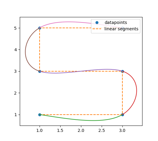
To calculate the length of the segments at each datapoint, we can use the formula that is described above.

\[s_i = \sum_{k=1}^i\sqrt{(x_{k+1}-x_{k})^2 + (y_{k+1}-y_{k})^2}\]

We now have an approximate length of the spline at each provided datapoint.

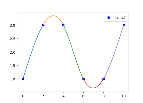
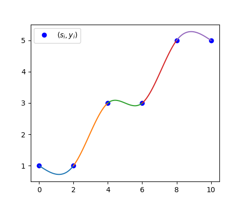
In the next step, we have to split the spline in two spline representations.

\[\begin{aligned} S_1: [s_i, x_i] &\to \mathbb{R}\\ S_2: [s_i, y_i] &\to \mathbb{R} \end{aligned}\]

To put it in other words, we will generate two splines, one with datapoints ($s_i$, $x_i$) and the other with the datapoints ($s_i$, $y_i$).
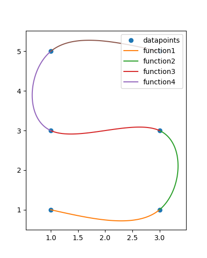
So in the end, we have two splines ($S_1$, $S_2$) that give us the x- and the y-coordinates for our parametrized spline. Since $s_i$ is strictly increasing, we will not get any problems which the spline cannot represent. Checkout the graphs below to see the two splines that make up the S shape spline (that I showed you above).

The source code is, as always, on GitHub. Check it out!

TL;DR

Spline parametrization is cool. Use it. Get the code on GitHub.

Man I love LaTeX in Markdown-Files ;)